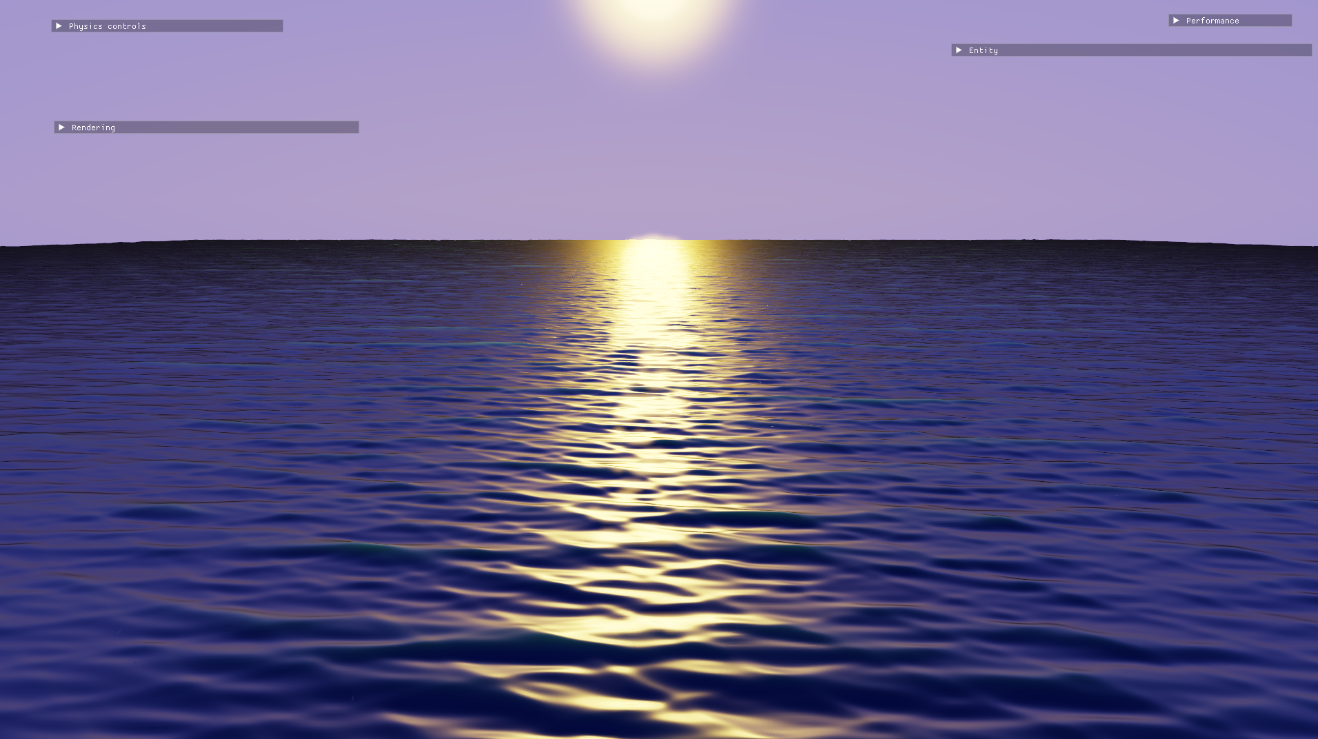
I set out to create a water rendering system for Gradient, my DirectX 11 renderer project. As someone new to graphics programming, diving into water rendering has been both exciting and challenging. This blog post shares my experience building my first water rendering system.
Wave modelling and generation
One of the most important components of water rendering is deforming a mesh to simulate waves convincingly. A water surface is typically modeled as a height field, where the height of the mesh at any given point is a periodic function of position and time. Acerola has an excellent video on the subject here. I decided to follow one of his references, Effective Water Simulation from Physical Models by Mark Finch. These techniques would be considered a bit dated by today’s standards, but I wanted to start from the basics.
Height function and normals
In GPU Gems, Finch starts with modelling waves as simple sums of sine waves and eventually goes on to discuss Gerstner waves. The problem with Gerstner waves, however, is that a poor choice of parameters can cause loops to form above the wave crests. To keep things simple, I chose to use sine waves where the sine function is offset to be non-negative and is raised to an exponent. This exponent can be used to control the sharpness of the peaks of the waves. In the interest of brevity, I’ll simply list the formulae here. A more complete treatment can be found in GPU Gems.
The height of the \(i\)th wave \(W_{i}(x,y,t)\) at position \((x,y)\) and time \(t\) is:
\[W_{i}(x,y,t)=2A_{i}\left(\frac{\sin(D_{i} \cdot (x,y) \times w_{i} + t\varphi_{i})+1}{2}\right)^{k}\]where
- \(A_{i}\) is the amplitude.
- \(D_{i}\) is the (two-dimensional) direction vector.
- \(w_{i}\) is the wave frequency.
- \(\varphi_{i}\) is the phase constant, which represents the speed of the crest of the wave.
- \(k\) controls the sharpness of the crests.
The height at any given point is the sum of all \(n\) waves:
\[H(x,y,t)=\sum_{i=0}^{n}W_{i}(x,y,t)\]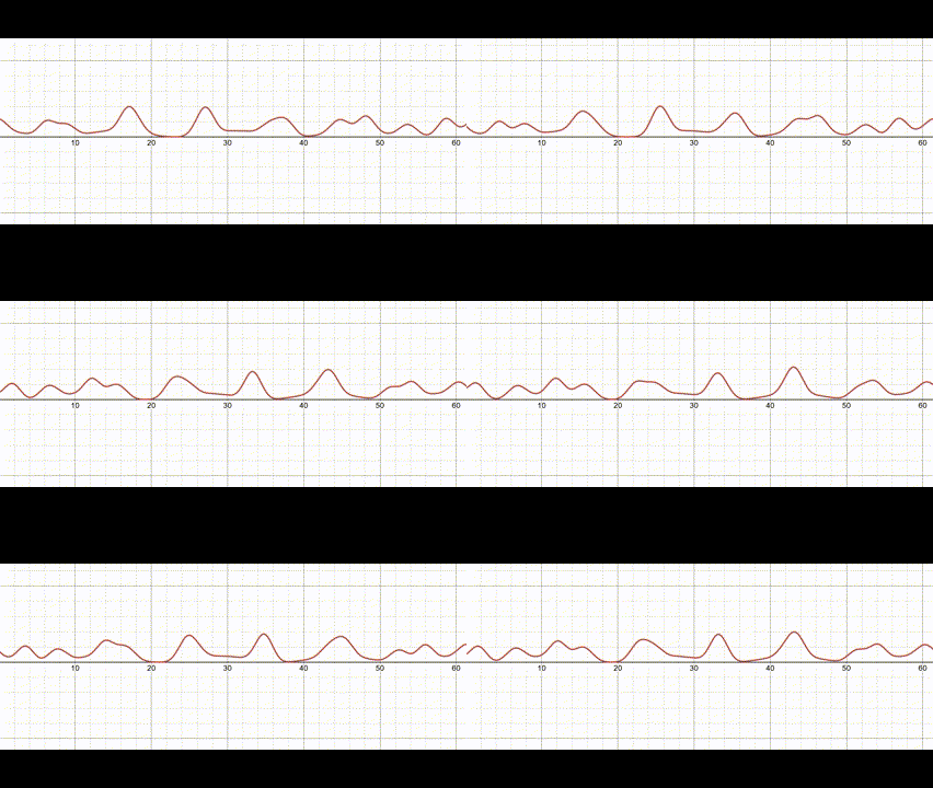
Waves modelled as a sum of sine functions. View this graph
To compute accurate lighting, I needed to calculate the normals for each point on the surface based on the height function. For any surface, the normal vector \(N(x,y)\) is the cross product of the binormal and tangent vectors at any point \((x,y)\). The binormal and tangent vectors are two orthogonal vectors that are tangential to the surface. Since the height function is an analytical function, the binormal and tangent vectors can also be computed analytically as the partial derivatives in the \(x\) and \(y\) directions respectively. The normal vector \(N(x,y)\) can then be computed as:
\[N(x,y)=\left( -\frac{\partial}{\partial x}H(x,y,t), -\frac{\partial }{\partial y}H(x,y,t),1 \right)\]The partial derivative of my wave function of choice \(W_{i}(x,y,t)\) is:
\[ \frac{\partial}{\partial x} W_i(x, y, t) = D_i.x \times w_i k A_i \left( \frac{\sin \left( D_i \cdot (x, y) \times w_i + t\varphi_i \right) + 1}{2} \right)^{k-1} \newline \times \cos \left( D_i \cdot (x, y) \times w_i + t \varphi_i \right) \]and the partial derivative for the total height function becomes:
\[ \frac{\partial }{\partial x}H(x,y,t)=\sum_{i=0}^{n}\frac{\partial }{\partial x}W_{i}(x,y,t) \]Generating the wave parameters
I modelled a single wave in HLSL as:
struct Wave
{
    float amplitude;
    float wavelength;
    float speed;
    float sharpness;
    float3 direction;
};
\(w_i\) can be computed from the wavelength as \(2 / wavelength\) and \(\varphi_i\) is \(speed \times w_i\). The other parameters can be readily plugged into the wave function formula. The y component of direction is unused, since Gradient uses a right-handed y-up coordinate system.
An array of these waves is generated on the CPU when the application starts up, and is passed to the shader in a constant buffer.
The direction of each wave is sampled from a normal distribution sampled around the wind direction. To prevent the total amplitude at any point from growing too high, the generated amplitude starts at a maximum value and is reduced for each successive wave. The speed of each wave is progressively increased and the sharpness is gradually reduced. From my testing, I found that 20 waves struck a nice balance between visuals and performance.
This is the complete wave generation code:
void WaterPipeline::GenerateWaves()
{
    float maxAmplitude = 0.1f;
    float maxWavelength = 5.f;
    float maxSpeed = 5.f;
    DirectX::SimpleMath::Vector3 direction{ -1, 0, 0.8 };
    direction.Normalize();

    std::random_device rd{};
    std::mt19937 gen{ rd() };

    std::normal_distribution xRng{ direction.x, 0.2f };
    std::normal_distribution zRng{ direction.z, 0.2f };

    float amplitudeFactor = 0.7f;
    for (int i = 0; i < m_waves.size(); i++)
    {
        auto d = DirectX::SimpleMath::Vector3{
            xRng(gen),
            0,
            zRng(gen)
        };
        d.Normalize();

        m_waves[i].direction = d;
        m_waves[i].amplitude = maxAmplitude * amplitudeFactor;
        m_waves[i].wavelength = std::max(0.2f,
            maxWavelength * amplitudeFactor);
        m_waves[i].speed = (1 - amplitudeFactor) * maxSpeed;
        m_waves[i].sharpness = std::max(1.f,
            std::round((m_waves.size() - (float)i)
                        * 16.f / m_waves.size()));

        m_maxAmplitude += m_waves[i].amplitude;

        amplitudeFactor *= 0.9;
    }
}
Mesh tessellation and displacement
To actually draw this height field to the screen, I can draw a flat plane mesh and then displace its vertices according to my height function. This mesh needs a large number of vertices or it would look jagged and uneven. Too many vertices, however, will result in poor performance.
Rather than generate the vertices ahead of time, I used DirectX 11’s tessellation shader pipeline to generate additional vertices on the fly. This allows me to control the amount of tessellation at runtime: the plane can be highly tessellated close to the camera to render fine details and less tessellated far away to improve performance.
Since the tessellation hardware has an upper limit on the amount of vertices it can generate for a given geometry patch, I couldn’t simply draw a single quad and tessellate it entirely on the fly. I generated a grid of triangles to be tessellated later.
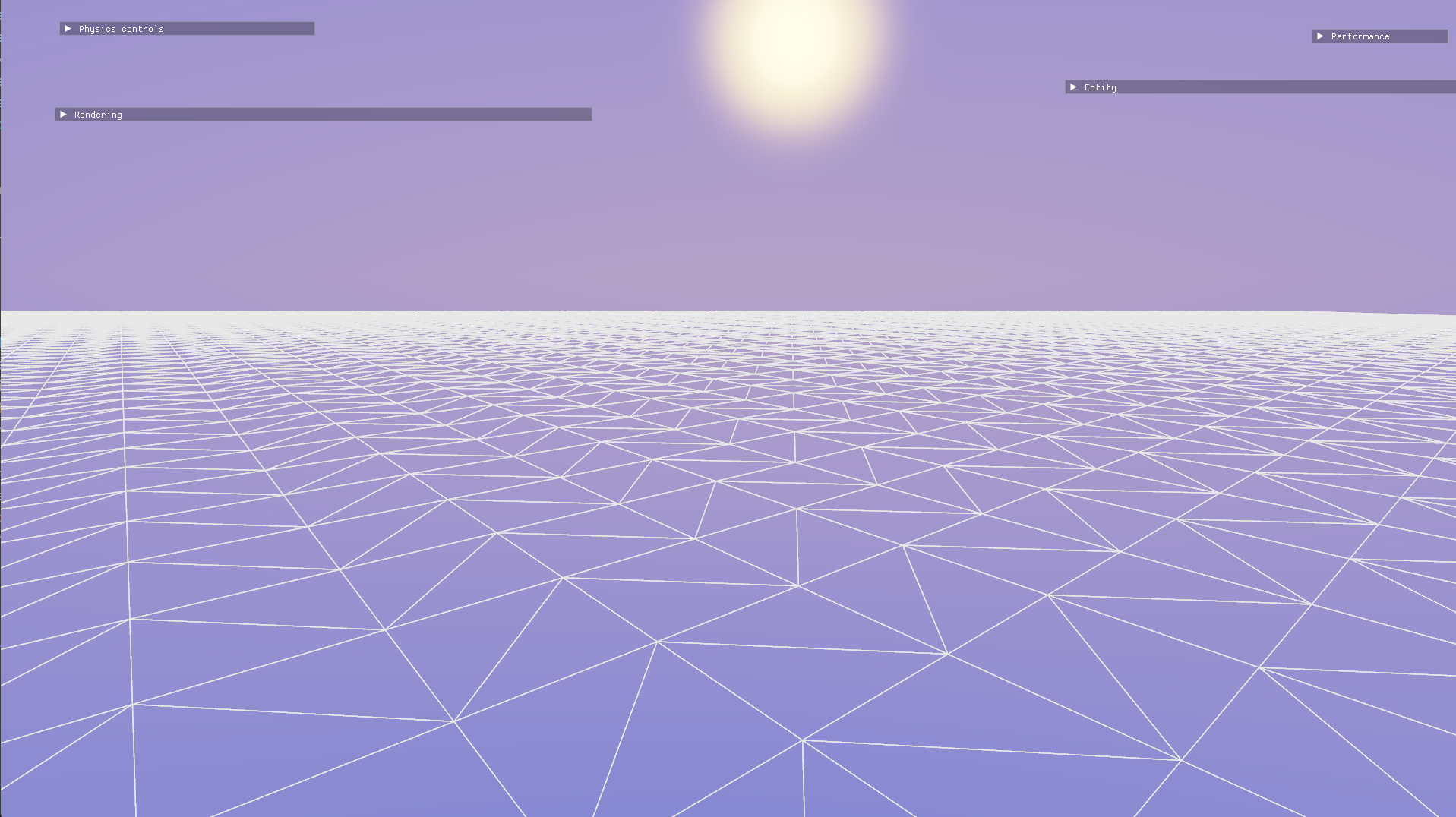
The starting grid, without any tessellation.
Frank Luna describes a distance-based tessellation method in his book Introduction to 3D Game Programming with DirectX 11. He starts by defining a minimum distance (below which patches are maximally tessellated) and a maximum distance (beyond which patches are not tessellated at all). He remaps this range to \([1..6]\) and uses the camera distance in this range as an exponent to the base 2. This value is used as the final tessellation factor. With this method, the tessellation factor varies exponentially with the camera distance in the range \([2^1..2^6]\) which is \([2..64]\).
float3 tessFactor(float3 worldP)
{
    const float d0 = g_minLodDistance; // Highest LOD
    const float d1 = g_maxLodDistance; // Lowest LOD
    const float minTess = 1;
    const float maxTess = 6;

    float d = distance(worldP, g_cameraPosition);
    float s = saturate((d - d0) / (d1 - d0));

    return pow(2, lerp(maxTess, minTess, s));
}
The tessellation factors are computed based on the midpoint of each edge. It’s important to compute tessellation factors based on properties of each edge only (as opposed to, say, using the midpoint of the patch) in order to prevent adjacent patches from having misaligned vertices.
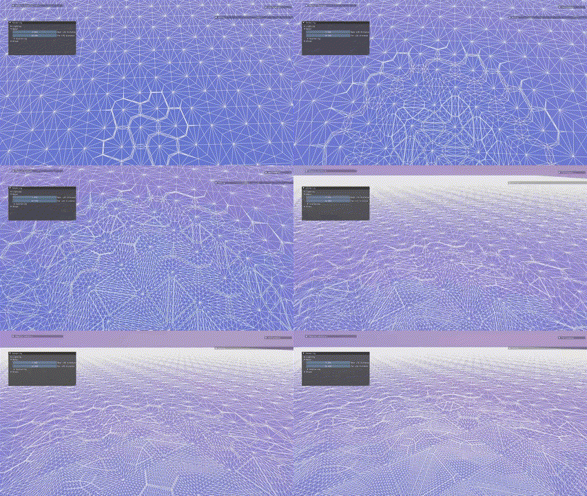
Distance-based tessellation. The tessellation distances have been reduced for illustration.
The height displacement and normal computation are done per tessellated vertex in the domain shader.
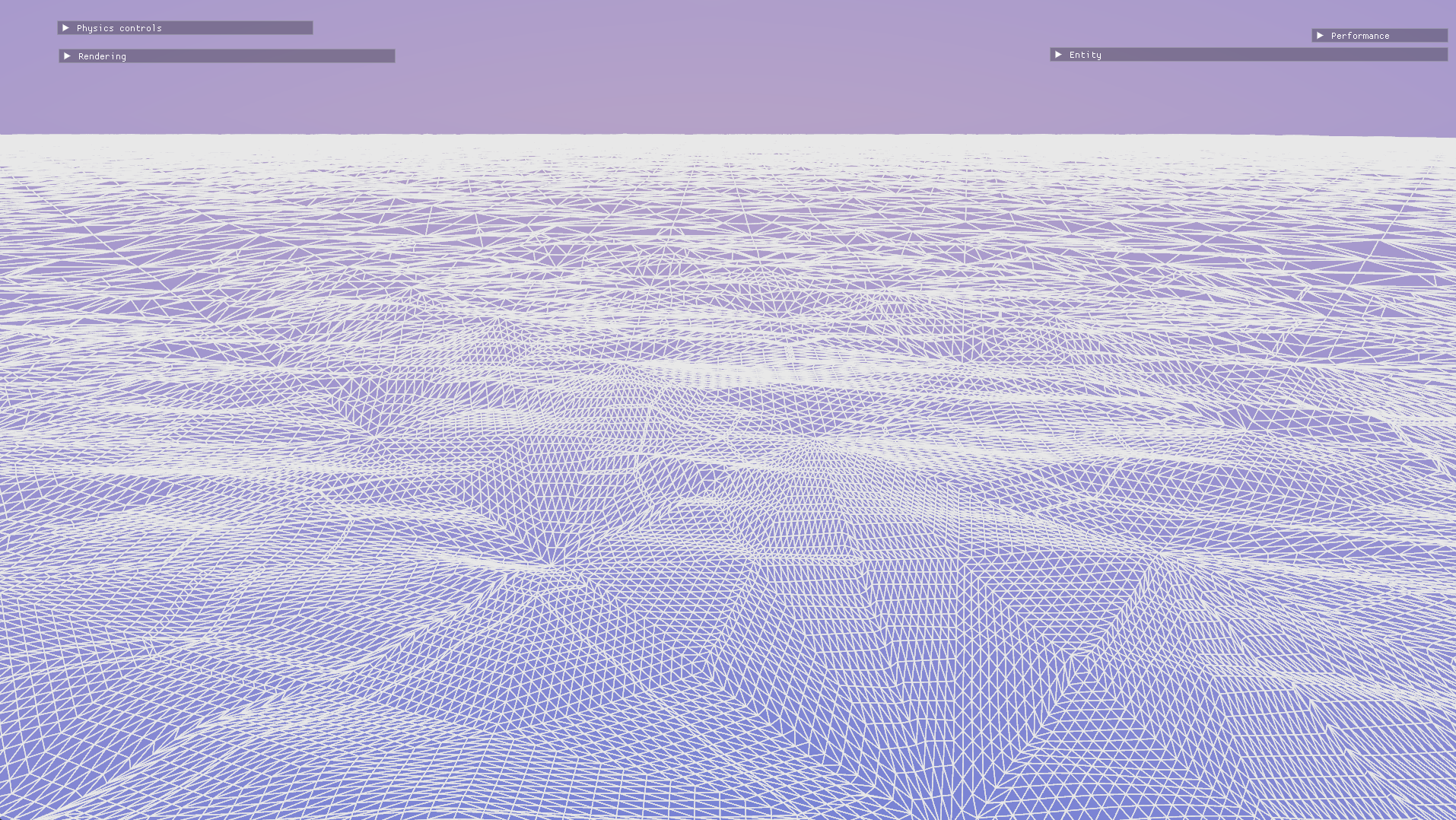
Displaced and tessellated vertices.
As a quick and dirty optimization, I culled patches that are behind the camera in the hull shader. It’s not quite as optimal as proper frustum culling, but it still improves performance by a lot and all it takes are a few dot products.
float3 toWorld(float3 local)
{
    return mul(float4(local, 1.f), g_worldMatrix).xyz;
}

float cameraDot(float3 worldP)
{
    return dot(normalize(worldP - g_cameraPosition),
               g_cameraDirection);
}

// ...

float3 e0 = toWorld(0.5 * (ip[0].vPosition + ip[1].vPosition));
float3 e1 = toWorld(0.5 * (ip[1].vPosition + ip[2].vPosition));
float3 e2 = toWorld(0.5 * (ip[2].vPosition + ip[0].vPosition));
float3 c = toWorld((ip[0].vPosition + ip[1].vPosition
                    + ip[2].vPosition) / 3.f);

Output.EdgeTessFactor[0] = tessFactor(e1);
Output.EdgeTessFactor[1] = tessFactor(e2);
Output.EdgeTessFactor[2] = tessFactor(e0);
Output.InsideTessFactor = tessFactor(c);

// Cull patches that are behind the camera.
float maxCameraDot = max(cameraDot(e0),
                max(cameraDot(e1),
                max(cameraDot(e2),
                    cameraDot(c))));

if (g_cullingEnabled && maxCameraDot < -0.1)
{
    Output.EdgeTessFactor[0] =
    Output.EdgeTessFactor[1] =
    Output.EdgeTessFactor[2] =
    Output.InsideTessFactor = 0;
}
With the displacement done, it’s now time to work on the lighting and visuals!
Pixel shading and visuals
PBR lighting
Gradient has a PBR (physically-based rendering) lighting system already, and I used this for my water shading. I’d like to cover my PBR lighting system in a later blog post, but for now, PBR is a modern approach to simulating realistic lighting based on the physical properties of materials. It focuses on how light interacts with surfaces like metals and non-metals. The three main parameters here are albedo, which is the base colour of a surface, roughness, which controls how bumpy or rough a surface appears and metallic, which determines whether the surface is a metal or not. Rougher surfaces are less reflective, and metals are much more reflective than non-metals.
Since water is a highly reflective surface, I set the roughness to a low value of 0.2 and the metallic to 1, indicating that the surface should be reflective like a metal. I set the albedo to (1, 1, 1), meaning that all colour would come through reflections. Gradient already has a cubemap-based reflection system for the sky dome. This causes the water surface to reflect the colours of the sky. Gradient also supports bloom as a post-process effect, and it looks great on the water surface.
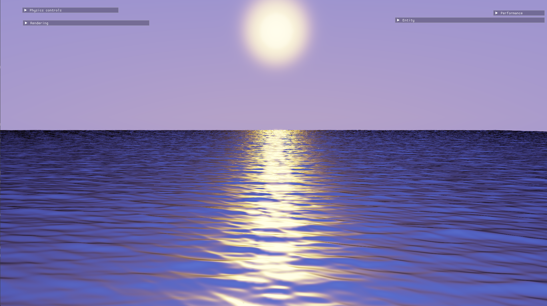
An early iteration of the water visuals.
This is a good start, but there’s a lot of noise on the water surface in the distance. (Admittedly, it’s hard to see in a compressed still, but trust me, it’s there.) To mitigate the noise, I interpolated the vertex normal with the up vector as the distance from the camera increases. This way, normals in the distance mostly point upward and don’t cause as much noise.
// Interpolate normals with the up vector
// as distance increases to reduce noise.
float3 lodNormal(float3 N, float3 worldP)
{
    const float d0 = g_minLodDistance;
    const float d1 = g_maxLodDistance;

    float d = distance(worldP, g_cameraPosition);
    float s = 1 - saturate((d - d0) / (d1 - d0));

    return lerp(float3(0, 1, 0), N, pow(s, 2.5));
}
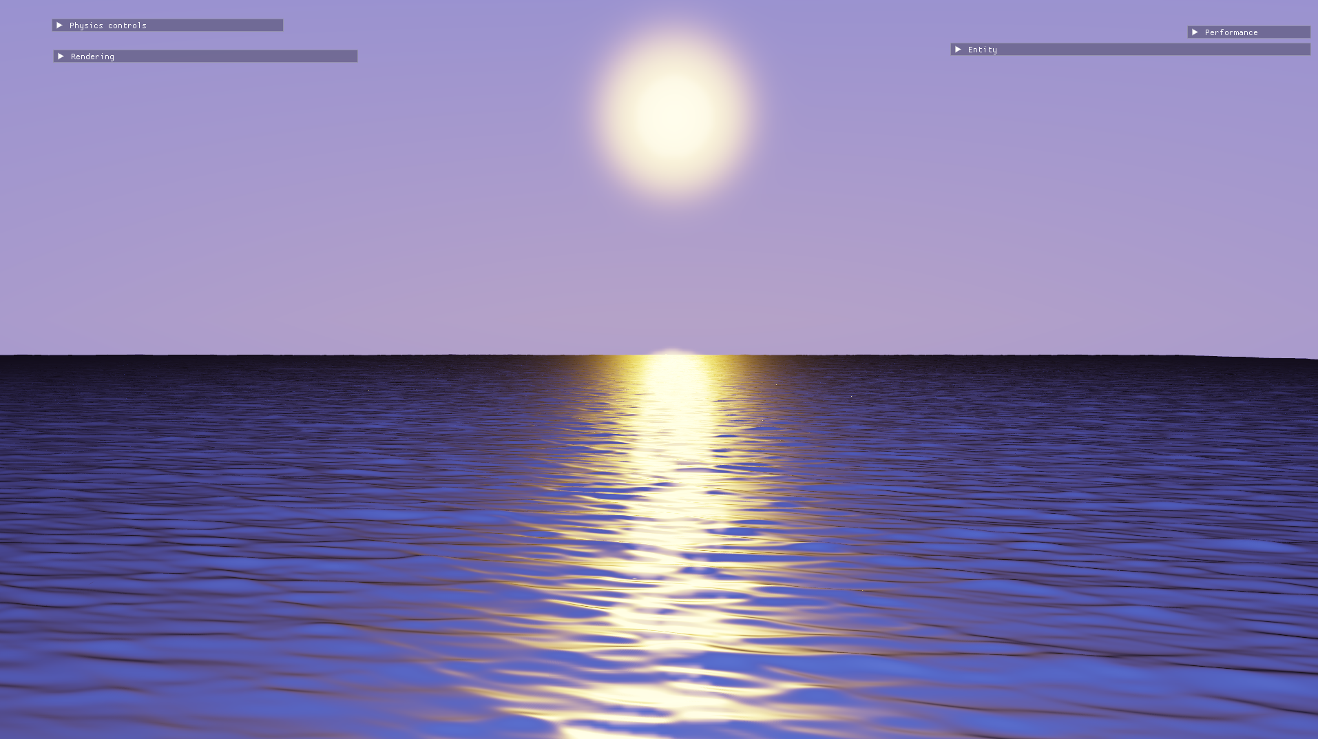
After interpolating normals with the up vector.
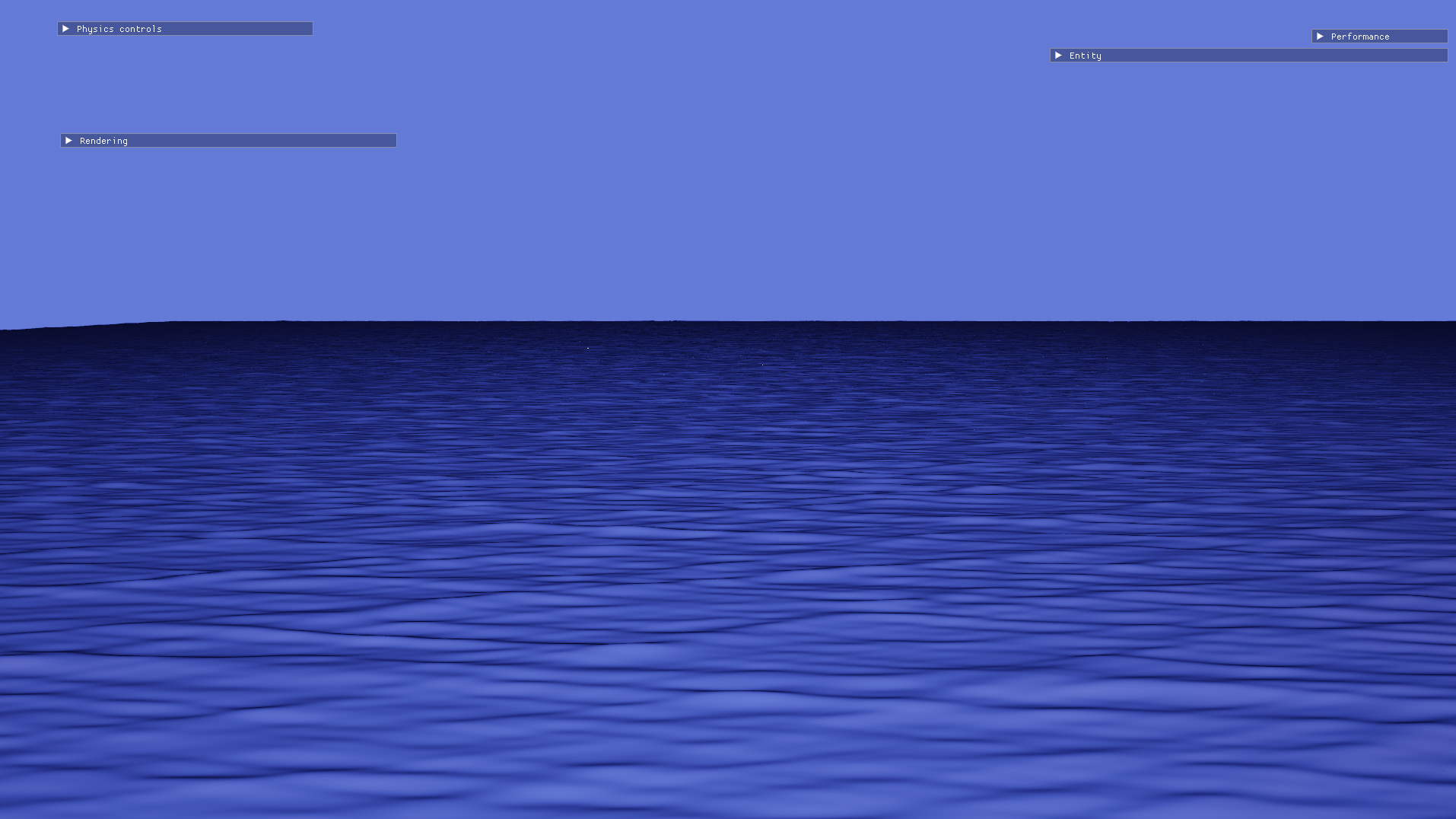
When facing away from the sun.
Subsurface scattering
Subsurface scattering occurs when light penetrates a surface, scatters within it, and exits at a different point, creating a soft glow effect. Subsurface scattering can be seen in a variety of materials, such as jade, skin and most importantly here, water. It’s an important component of water rendering since it helps add a sense of translucency.
Though there are many sophisticated approaches to rendering subsurface scattering, I was short on time and I wanted a method that was easy to implement, even if it wasn’t the most realistic. I came across a simple approach by Alan Zucconi, which was in turn inspired by the talk Approximating Translucency for a Fast, Cheap and Convincing Subsurface Scattering Look by Colin Barré-Brisebois and Marc Bouchard. I used this method, with a few tweaks. The general idea behind his method is that in translucent materials, some light passes through the object and ends up illuminating the side of the object that is facing away from the light. Thus, if \(L\) is the unit vector from a point on the surface in the direction of incident light, there is also a small lighting contribution from the direction of \(-L\). To account for refraction, \(-L\) is adjusted towards the surface normal a little bit. The amount of light transmitted also depends on the distance travelled by the light through the surface: the greater the distance travelled, the less light will be transmitted. I approximated this with a simple thickness parameter ranging between 0 (all light is transmitted) and 1 (no light is transmitted). Here’s my subsurface scattering code:
// Simple thickness-based subsurface scattering,
// inspired by https://www.alanzucconi.com/2017/08/30/fast-subsurface-scattering-1/
float3 subsurfaceScattering(float3 irradiance,
                            float3 N,
                            float3 V,
                            float3 L,
                            float thickness,
                            float sharpness,
                            float refractiveIndex)
{
    float I = (1 - thickness)
        * pow(saturate(dot(V,
                           normalize(-L + N * (refractiveIndex - 1)))),
              sharpness)
        * 0.05;

    return I * irradiance;
}
Where:
irradianceis the HDR colour of the incoming light.Nis the normal vector.Vis the unit vector from the point to the camera (the view vector).Lis the light vector as described above.refractiveIndexis a parameter governing the adjustment of transmitted light towards the normal - values greater than 1 cause the light to bend towards the normal.sharpnessgoverns how narrowly transmitted light is scattered outwards.thicknessrepresents the thickness of the surface, ranging from0to1.
But the question remains - how can thickness be determined at any given pixel? Again, I wanted a quick solution that looked good enough rather than perfect photorealism. I decided to approximate thickness based on how high the pixel was on a wave. The rationale here is that waves have a lower thickness or cross-sectional area from bottom to top.
// Using the height here as a proxy for thickness.
// The peaks of each wave are thinner than
// the troughs.
float heightRatio = saturate(input.worldPosition.y / g_maxAmplitude);
float thickness = 1 - pow(heightRatio, g_thicknessPower);
thicknessPower is yet another parameter I used to tweak how far up on the wave the thickness started to reduce.
For each light in the scene, I computed the subsurface scattering contribution and added it to the total lighting of a pixel on the water. This is the result after some parameter tweaking:
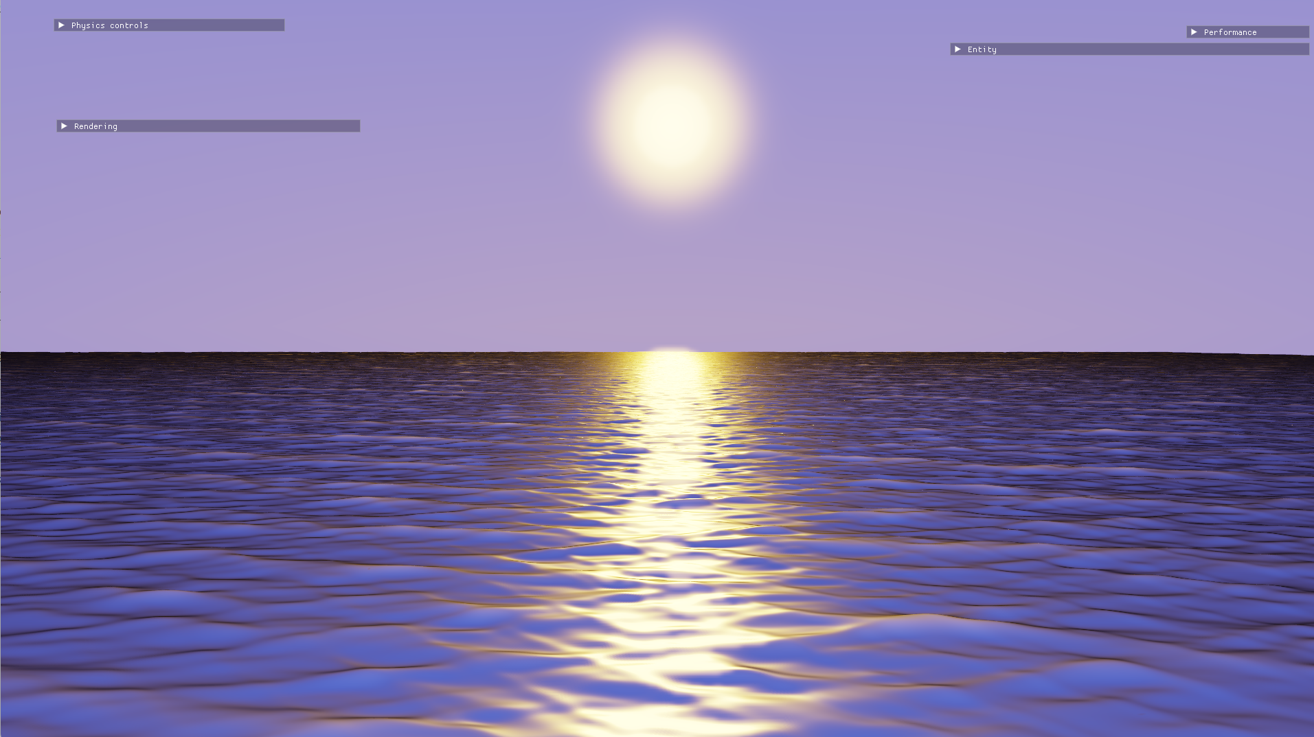
The first iteration of subsurface scattering.
There’s now a gentle glow at the tip of each wave. It’s not photorealistic, but I still quite like it! I think it helps emphasise the shape of the waves, especially in the distance.
The Fresnel effect, and improved subsurface scattering
The water still doesn’t look quite right, though. The surface looks completely opaque - it somehow doesn’t have that sense of depth or translucency like real water.
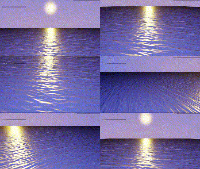
What am I missing?
This problem had me stumped. Gradient isn’t simply a side project, however - I was to submit it as my university coursework, and I was on a deadline. So at this point, I decided to stop working on the water and move on to other features, with the intention of working on the water later after I was done with my submission.
After the semester ended, I came across a large lake while on holiday. Here, I made some observations about the water’s appearance that would lead to a breakthrough.
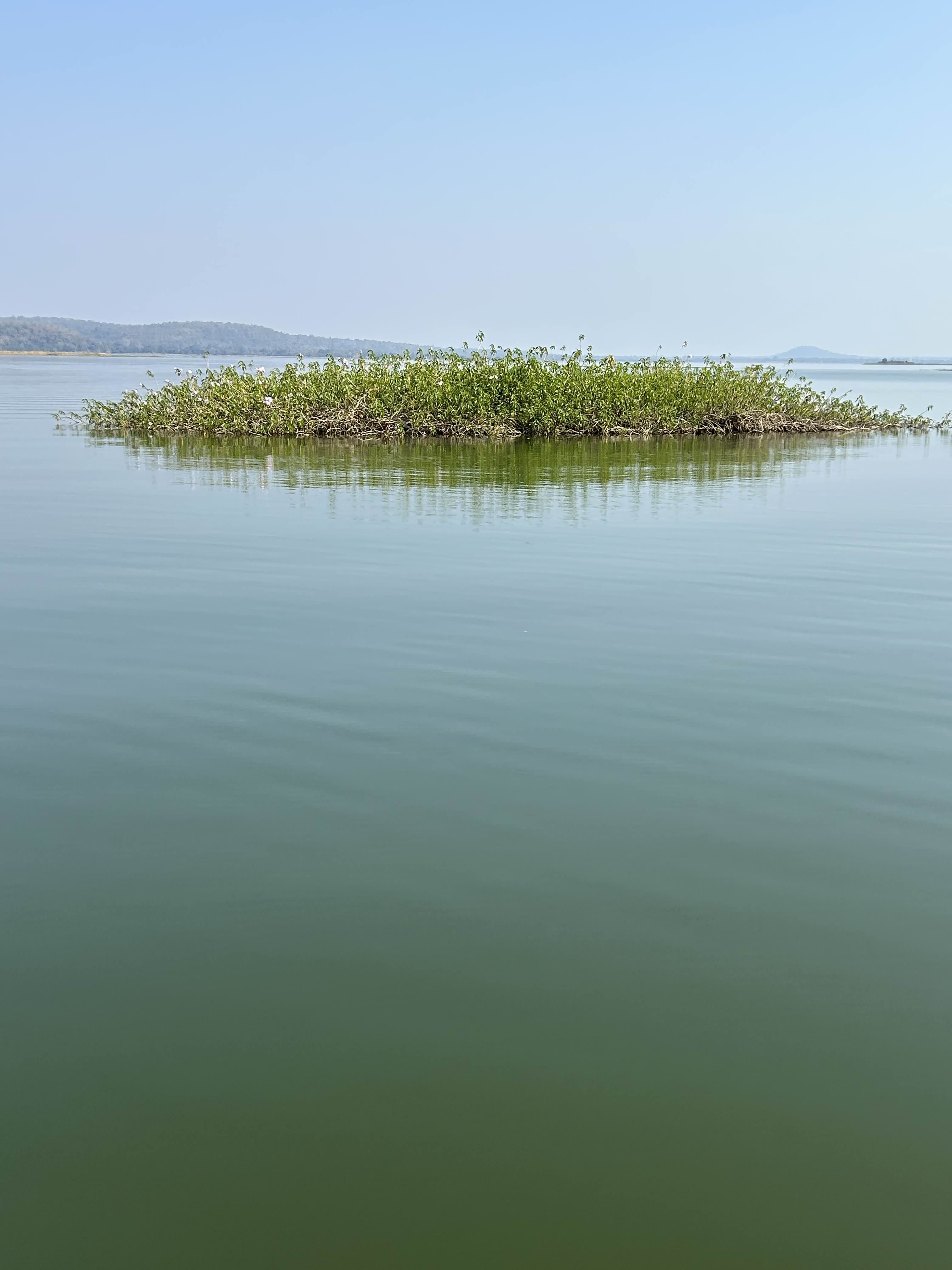
Aha!
The lake surface is very reflective, unless I’m looking straight down into it! When looking straight down into the water, it transmits this greenish-blue colour. In more technical terms - the water surface is highly reflective at grazing view angles but is more translucent as the view vector approaches the surface normal. The tendency for materials to be highly reflective at grazing angles is known as the Fresnel effect.
To simulate this effect, I chose a colour for deep water and interpolated the albedo between the water colour and pure white (fully reflective) based on the viewing angle. Separately, I also decided to multiply the subsurface scattering contribution by a shallow water colour to make the glow bluish rather than white.
// The colour transmitted by shallow water
float3 shallowWaterColour = float3(0.14, 0.94, 0.94) * 0.5;
// The colour transmitted by deep water
float3 deepWaterColour = float3(0.06, 0.11, 0.19) * 0.5;
// Water is more reflective at grazing view angles and
// more transmissive at oblique angles.
float reflectanceFactor = pow(1.f - pow(max(dot(N, V), 0), 2.5),
                              5);

float3 albedo = lerp(deepWaterColour, float3(1, 1, 1),
                     reflectanceFactor);
I computed the reflectance factor using a modification of Schlick’s Fresnel approximation. Raising \(N \cdot V\) to an exponent has the effect of limiting the “radius” of the dark patch around the camera.
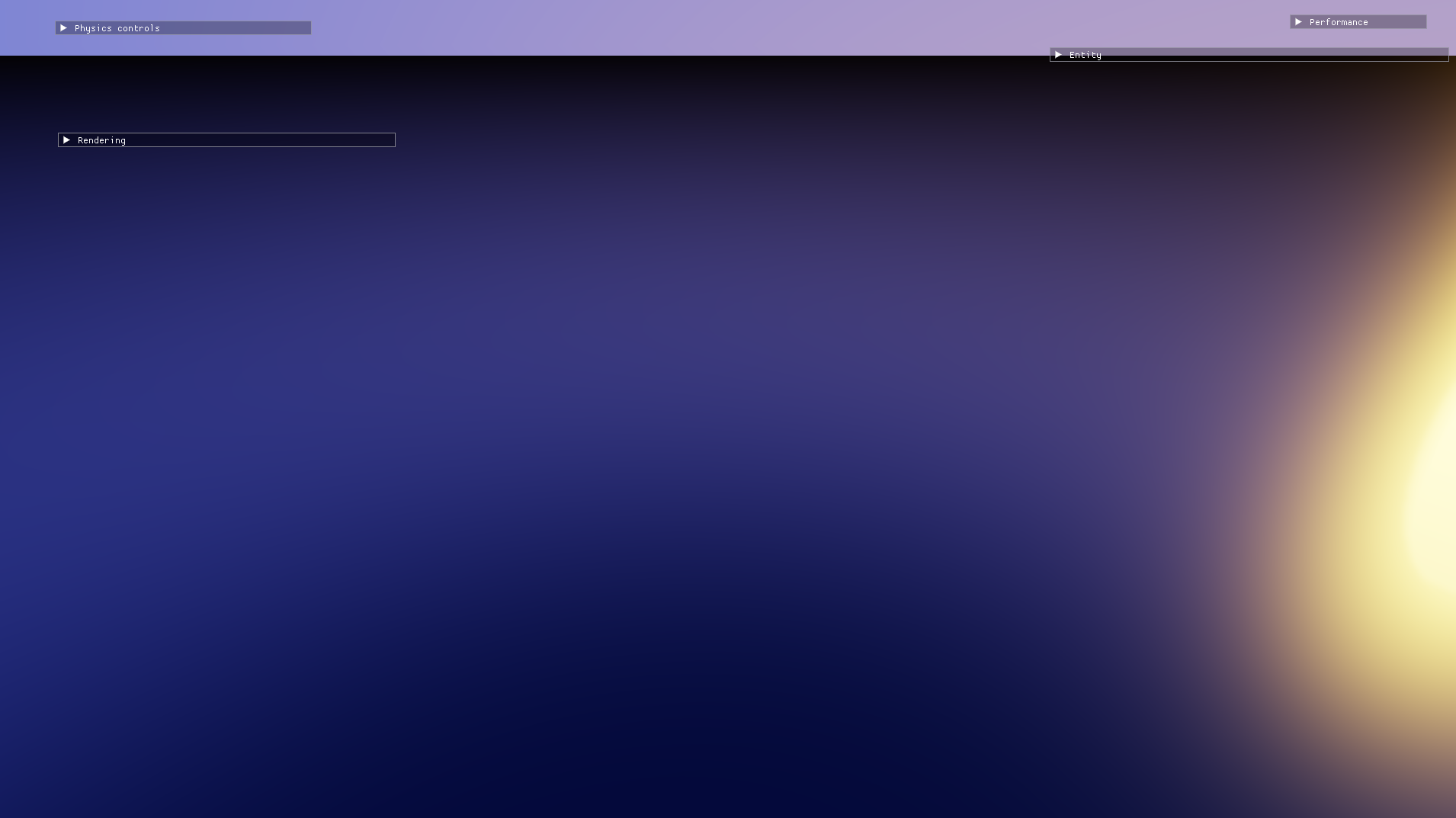
The effect on a surface without any wave animation. Notice the dark patch near the camera.
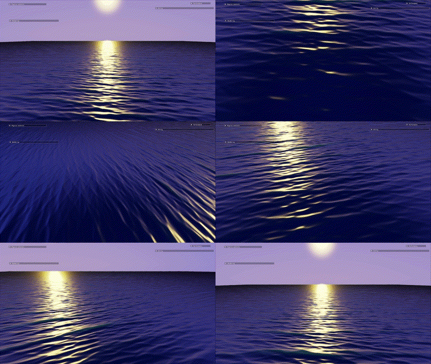
The effect on the animated water surface.
Much better! The new shader properly conveys a sense of depth when looking straight down into the water.

The final water visuals.
Reflections (ha!) and scope for improvement
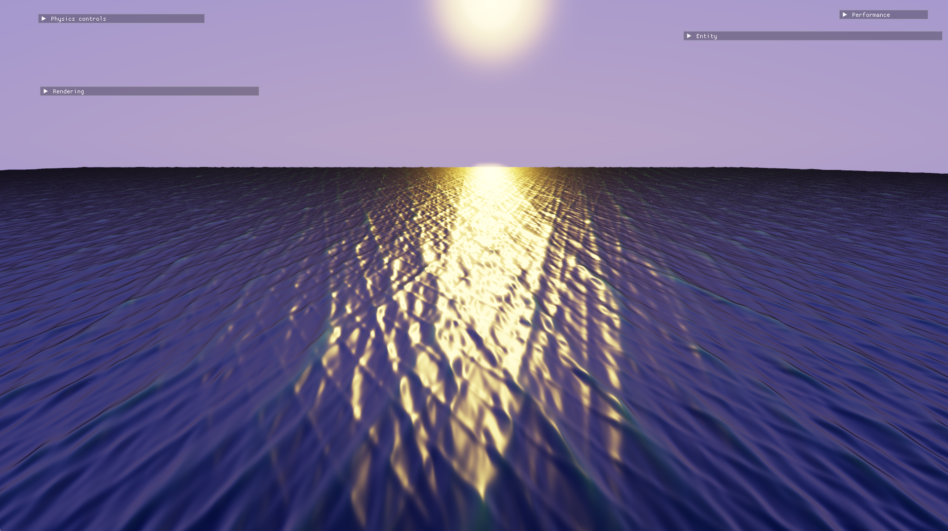
The tiling on the water is quite obvious from certain angles.
There are still many issues with this water simulation:
- The actual reflections on the water surface are currently quite unremarkable. This is because i) the water is only reflecting the sky dome and ii) the sky dome itself doesn’t really have any details such as clouds. Adding planar or screen-space reflections to the water surface and some details to the sky would make the visuals much more impressive.
- The water lacks finer detail when viewed up close. I could simply scroll a normal map over the water surface to alleviate this.
- There’s some very visible tiling, especially when viewing the water at an angle orthogonal to the wind direction. Adding more waves to the sine wave sum could mitigate this issue but it would be prohibitively expensive past a point. The water surface also lacks other details such as foam and choppiness. Tessendorf’s approach to water simulation using a fast Fourier transform (FFT) is much more sophisticated and realistic, and this technique is used today in Sea of Thieves.
- I would like to explore moving normal computation from the domain shader to the pixel shader. It’s hard to predict what impact this would have on performance. On the one hand, this would allow me to get away with less tessellation since normals are computed per-pixel anyway. On the other hand, computing normals per pixel could be even more expensive, especially at higher resolutions.
Given that this is my first attempt at a water simulation though, I’m quite happy with the results!